Answer: Skip the leading 1 and read the remaining digits from left to right: every digit means square, and every 1 also means multiply by .
Fiddling with Fibonacci
Here’s a riddle: I am a number. I start with 1953282128 and end with 8242546875. In between are another 208,968 digits. What am I? The answer: the millionth Fibonacci number, of course! By the end of this post you’ll be able to compute it in a seventh of a second. Not with a supercomputer or a sophisticated library, but with a few lines of Python and one beautiful idea. But first, let’s take a step back.
The rabbit hole
You’ve probably met this sequence before:
Every number is the sum of the two before it. Formally:
starting from the base condition
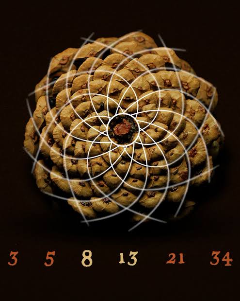
The sequence is famous for its relation to the Golden ratio, a proportion that hides in the patterns of sunflower seeds, pine cones and many other beautiful displays of Nature. But today we only care about one thing: to compute the millionth Fibonacci number. Why? Not because we care about the result, but because solving this exercise allows one to reinvent some of the most powerful, elegant and fundamental concepts in computational problem-solving.
1. Plain recursion: the million-year program
Because the Fibonacci sequence is defined via a recursive relation, the simplest way to compute it uses a recursive algorithm.
def fib(n):
    # Base case
    if n == 0:  return 0
    if n == 1:  return 1

    # Recursion
    return fib(n-1) + fib(n-2)
Isn’t it beautiful? It almost feels like cheating: the algorithm that computes the sequence is identical to its own very definition. But you can easily try for yourself that it really works! Despite its elegance, unfortunately, this algorithm is also catastrophically slow! Just have a look at the table below:
| Target | Calls | Time (30 million calls per second) |
|---|---|---|
fib(30) | 2.7 million | 90 ms |
fib(40) | 331 million | 11 s |
fib(50) | 41 billion | 22 min |
fib(100) | 1.1 × 10²¹ | 1.2 million years |
And we want the millionth.
The issue is that every call to fib(n) generates two additional function calls, such that the number of calls doubles for every next number along the sequence. The algorithm is doing a lot of the same work multiple times: fib(n-2) gets computed once directly, and then all over again inside fib(n-1). Further down the tree, the same small values are recomputed billions of times.
2. Caching up to speed: from millions of years to milliseconds
Fortunately, there is a very simple fix. All we need to do is check - before running an expensive computation - whether we have already solved this problem before. In other words, we need to remember our solutions. This is done using a cache: a variable that stores the result of a computation.
cache = {}

def fib(n):
    if n == 0:  return 0
    if n == 1:  return 1
    if n not in cache:
        cache[n] = fib(n-1) + fib(n-2)
    return cache[n]
Now, each fib(n) is only computed once. On the second call, it just looks up the answer from the cache.
| Target | Calls | Time (30 million calls per second) |
|---|---|---|
fib(30) | 59 | 2 µs |
fib(40) | 79 | 3 µs |
fib(50) | 99 | 3 µs |
fib(100) | 199 | 7 µs |
fib(1000) | 1,999 | 67 µs |
fib(1,000,000) | 2 million | 67 ms |
One snag: in addition to time, we also have to think about memory. Every function call requires memory to execute, and this memory can only be vacated after the function completes its calculation. But fib(n) can’t finish until fib(n-1) has finished, which can’t finish until fib(n-2) has finished, and so on all the way down to fib(1). So at the deepest point, unfinished calls are stacked on top of each other, all waiting. In addition, our solver must remember the result of each of those one million function calls. This means that, to compute fib(1,000,000), the cache alone would take up about 43 GB of storage; the space needed to store all Fibonacci numbers below one million (as we have seen, those numbers get very big). Hence, not time but memory is now the main obstacle.
3. Walking up the stairs: a bottom-up approach
So let’s turn it around. Instead of starting at the top and recursing down, we can also start at the bottom and climb up, carrying only the last two numbers:
def fib(n):
    a, b = 0, 1
    for i in range(n):
        a, b = b, a+b
    return a
No recursion, no cache, barely any memory. And for the first time, the millionth Fibonacci number is within reach: computing it takes about 5 seconds. That feels like the end of the road. Each number needs the one before it, so surely you have to take all steps?
You don’t.
4. Matrix powers: taking the elevator
Let’s take a quick detour, to the simplest recursion imaginable:
1, 2, 4, 8, 16, 32, etc. Each number is twice the previous one, starting at 1. Nobody would compute this step by step. We just see the pattern:
The above formula allows one to compute any number in the sequence directly, i.e. without needing to calculate all the numbers before it. Here comes the beautiful part: this trick still works when is a matrix instead of a number. Now watch as the magic unfolds. I begin by writing down two equations. The first is the definition of our problem, the second is a trivial one that seems useless for now.
Now we rewrite this system of equations using matrix notation. Nothing special here, just a different notation.
Now notice how this starts to resemble the form . One multiplication by that little 2x2 matrix moves us one step along the sequence, just like multiplying by 2 did for . Starting from and , we take steps:
The whole Fibonacci sequence, folded into a single matrix power. On its own, that’s still multiplications. The magic is that powers don’t have to be computed one step at a time.
Squaring our way there
How would you compute ? Not as , but by squaring:
Hence we do followed by and finally to arrive at the answer. Three multiplications instead of seven. But a million isn’t a neat power of 2, so how do you find the route there? The trick is to work backwards, let’s just the number thirteen as an example.
The above diagram shows us how we can efficiently raise a number to the power thirteen:
That’s it, now we have everything we need. Following this process, the millionth Fibonacci number only requires 31 matrix multiplications. The code below shows you how to do it, and completes in about a seventh of a second.
Bonus: to quickly figure out when to square and when to multiply, we can use a neat little trick involving the binary representation of our number. For example, in binary, 13 is 1101. Can you figure out how this helps us square our way to a desired exponent?
Reveal the answerHide
Recapitulating
We have learnt the following key lessons when it comes to solving recursive problems:
- A recursive algorithm is often the easiest to implement.
- Through caching one can achieve a dramatic speed up at the cost of memory.
- bottom-up approaches generally perform better than top-down (recursive) algorithms.
- If you can reformulate your problem using matrices, magical things tend to happen.
That said, the next time you encounter a difficult problem, I don’t recommend immediately trying the most efficient solution involving matrices. In my experience, it is generally best to follow a journey like we have done here: starting with something simple that works and making improvements where necessary. This way, the simple solutions can be used to validate the efficient solutions, and you are far less likely to get stuck.
Hope you enjoyed reading this article and learned something in the process. Catch you in the next one!
-Kasper
def fib(n):
    if n == 0:  return 0
    return mat_pow([[1, 1], [1, 0]], n-1)[0][0]

def mat_pow(M, n):
    """M to the power n"""
    if n == 0:  return [[1, 0], [0, 1]]   # M^0 (the identity matrix)
    result = M                            # The leading 1
    for digit in bin(n)[3:]:              # The remaining digits, e.g. 13 -> '101'
        result = mat_mul(result, result)
        if digit == '1':
            result = mat_mul(result, M)
    return result

def mat_mul(X, Y):
    """Multiply two 2x2 matrices"""
    return [
        [X[0][0]*Y[0][0] + X[0][1]*Y[1][0], X[0][0]*Y[0][1] + X[0][1]*Y[1][1]],
        [X[1][0]*Y[0][0] + X[1][1]*Y[1][0], X[1][0]*Y[0][1] + X[1][1]*Y[1][1]],
    ]

if __name__ == '__main__':
    x = fib(1_000_000)
    # >>> import sys; sys.set_int_max_str_digits(0)  # Allow printing large numbers
    # >>> print(x)
    # ... 1953282128...8242546875